What Inflation Does

The path planner treats the robot as a point. That is what lets it solve the shortest-path problem efficiently on a cell-to-adjacent-cell graph. But a real robot has width. Inflation is the elegant trick that resolves this contradiction.

Shifting the Robot's Size onto the Obstacles

The idea is simple. If the robot has width, inflate the obstacles by that width. Then, as long as the point-robot does not touch an inflated obstacle, the physical robot will not touch the real obstacle.

Rendering diagram…

The inflation layer places concentric cost rings around lethal cells (obstacles), decaying exponentially with distance.

Distance:   0      r_robot        inflation_radius
Cost:      254  →  ~mid cost  →  0
           (lethal) (risky zone)   (free)

• Inside the inscribed radius — robot center entering here always means collision → effectively lethal
• Between inscribed radius and inflation_radius — passable but expensive (cost↑) → planner avoids it
• Beyond inflation_radius — cost 0, free space

Written as pseudocode, the rule is easy to grasp at a glance — each free cell's cost is determined by a single value: the distance to the nearest obstacle.

LETHAL = 254  # effectively a collision

def inflation_cost(distance, robot_radius, inflation_radius, decay=3.0):
    # distance = distance from this cell to the nearest obstacle
    if distance <= robot_radius:          # (1) inside the inscribed radius
        return LETHAL                     #     → always a collision
    if distance <= inflation_radius:      # (2) inside the bloated region
        # decays exponentially with distance
        return round((LETHAL - 1) * exp(-decay * (distance - robot_radius)))
    return 0                              # (3) beyond = free space

distance is typically computed for all cells at once via a distance transform. The key point — cost is a function of distance. That is exactly why you get the concentric gradient that falls smoothly to 0 the farther you get from an obstacle.

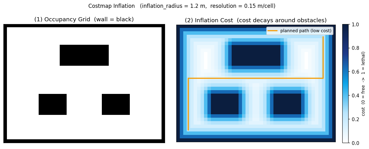Occupancy grid (left, walls=black) bloated to inflation_radius=1.2 m (right). Cost decays from lethal outward in concentric rings (cyan→white); the path planner routes through the center of low-cost corridors (orange path).

This gradient naturally steers the robot toward the middle of corridors rather than hugging walls. The orange path in the figure above follows that low-cost valley.

▶ Simulation footage — Clearpath AMR navigating a warehouse aisle. The occupancy grid, costmap, and inflation described here all combine to produce this behavior.

Where the Radius Comes From — and the Heterogeneous Fleet Problem

inflation_radius is set by multiplying the robot's radius by a safety factor (we typically use radius × 1.5). The robot radius is read from each robot's manifest — a small AMR and a large transport robot must have different values.

This is where multi-robot deployments hit a wall.

Rendering diagram…

When robots of different sizes (e.g., a compact AMR and a large Husky) share one costmap, there is only one inflation radius. Setting it large (for the big robot) causes the small robot to see passable corridors as blocked and stall. Setting it small (for the small robot) allows the large robot to clip walls. We observed exactly this behavior — a large robot stalling in a narrow passage — and the root cause was that inflation was not per-robot.

This is a clean illustration of the too-large vs. too-small trade-off. The correct answer is per-robot footprints; sharing a single costmap is only safe in homogeneous fleets.

In a nutshell

📌 Inflation = bloating obstacles by the robot's width so the path planner can treat the robot as a point. The radius comes from the robot manifest; inflation_radius = robot_radius × 1.5 is the common default. Because a costmap carries only one radius, heterogeneous fleets require per-robot footprint separation.